General Plotting routines
The plotting of data is always a common task that needs to be performed. However, there is a lot of variation in how someone might want plots to look or be arranged. Some plots might also need to be interactive to be of a real use.
For these reasons the masci_tools library provides utility for general plotting and
template functions for common plots made when working with DFT methods.
There are two plotting backends available:
matplotlib: Mainly used for non-interactive plots
bokeh: Mainly used for interactive plots
Available Routines
For both of these there are a lot of plotting routines available (both general or specific
to a problem). All of these routines will return the used Axes object in the
case of matplotlib or the figure produced by bokeh for custom modifications.
common (Can be used for both backends):
scatter(): Make a scatterplot with varying size and color of the points for multiple sets of dataline(): Make a lineplot with multiple sets of datados(): Plot a general density of states (non-spinpolarized)spinpol_dos(): Plot a general density of states (spinpolarized)bands(): Plot a general bandstructure (non-spinpolarized)spinpol_bands(): Plot a general bandstructure (spinpolarized)
matplotlib:
single_scatterplot(): Make a scatterplot with lines for a single set of datamultiple_scatterplots(): Make a scatterplot with lines for multiple sets of datamulti_scatter_plot(): Make a scatterplot with varying size and color of the points for multiple sets of datacolormesh_plot(): Make 2D plot with the data represented as colorwaterfall_plot(): Make 3D plot with thescatter3Dfunction of matplotlibsurface_plot(): Make 3D plot with theplot_surfacefunction of matplotlibmultiplot_moved(): Plot multiple sets of data above each other with a configurable shifthistogram(): Make a histogram plotbarchart(): Make a barchart plotmultiaxis_scatterplot(): Make a plot containing multiple sets of data distributed over multiple subplots in a gridplot_convex_hull2d(): Make a 2D plot of a convex hullplot_residuen(): Make a residual plot for given real and fit data. Can also produce a histogram of the deviationsplot_convergence(): Plot the convergence behaviour of charge density distances and energiesplot_lattice_constant(): Plot the energy curve with changing unit cell volumeplot_dos(): Plot a general density of states (non-spinpolarized)plot_spinpol_dos(): Plot a general density of states (spinpolarized)plot_bands(): Plot a general bandstructure (non-spinpolarized)plot_spinpol_bands(): Plot a general bandstructure (spinpolarized)plot_spectral_function(): Plot a spectral function (colormesh along kpath)
bokeh:
bokeh_scatter(): Make a scatterplot for a single set of databokeh_multi_scatter(): Make a scatterplot for a multiple sets of databokeh_line(): Make a line plot for multiple sets of databokeh_dos(): Plot a general density of states (non-spinpolarized)bokeh_spinpol_dos(): Plot a general density of states (spinpolarized)bokeh_bands(): Plot a general bandstructure (non-spinpolarized)bokeh_spinpol_bands(): Plot a general bandstructure (spinpolarized)bokeh_spectral_function(): Plot a spectral function (colormesh along kpath)periodic_table_plot(): Make a interactive plot of data for the periodic tableplot_lattice_constant(): Plot the energy curve with changing unit cell volumeplot_convergence(): Plot the convergence behaviour of charge density distances and energiesmatrix_plot(): Plot a grid of rectangles with color scaling and added text
If you have ideas for new useful and beautiful plotting routines you are welcome to contribute. Refer to the sections Using the Plotter class and Using the PlotData class for a guide on how to get started.
Providing Data
Data can be provided to plotting functions in two main ways:
The first arguments and data arguments are given the keys in a mapping, which should be used. The corresponding mapping is provided via the
datakeyword argumentThe first arguments and data arguments are given the data that should be plotted against each other.
The following two code blocks are equivalent in terms of the provided data.
from masci_tools.vis.plot_methods import multiple_scatterplots
import numpy as np

x = np.linspace(-10,10,100)
y1 = x**2
y2 = 20*np.sin(x)

#The data is split up according to fixed rules that the plot function defines.
#The default behaviour is that a list of lists is interpreted as multiple separate plots
ax = multiple_scatterplots(x, [y1, y2])
from masci_tools.vis.plot_methods import multiple_scatterplots
import numpy as np

x = np.linspace(-10,10,100)
y1 = x**2
y2 = 20*np.sin(x)
data = {'x': x, 'y1': y1, 'y2': y2}

ax = multiple_scatterplots('x', ['y1', 'y2'], data=data)
Customizing Plots
You might want to change the parameters of your plot. From changing the color,
linestyle or shape of the markers there are a million options to tweak.
These can be set by simply passing the keyword arguments with the desired parameters
to the plotting function. The names of these parameters mostly correspond to the
same names as in the plotting library that is used in the plotting function.
However, there are some deviations and also some special keywords that you can use.
We will go over the most important ones in this section accompanied with concrete code
examples. For a reference of the defaults defined in the masci_tools library you can
refer to matplotlib_plotter.MatplotlibPlotter and
bokeh_plotter.BokehPlotter for a complete reference.
The most important special keywords are listed below. If there are deviating names for
these in matplotlib and bokeh plotting functions both names are written in the
order matplotlib or bokeh:
limits: This is used to set the bounds of the axis specifically. Provided in form of a dictionary. For example passinglimits={'x': (-5,5)}will set the x-axis limits between-5and5andlimits={'x': (-5,5), 'y':(0,10)}will set the y-axis limits in additionscale: Used to set the scaling of the axis in the plots. Also provided in form of a dictionary. For example passingscale={'x': 'log', 'y': 'log'}will set both axis to logarithmic scalingscale={'y': 'log'}will only to it for the y-axislinesorstraight_lines: Easy way to draw help lines into the plot. Provided in form of a dictionary. For example passinglines={'vertical': 0}will draw a vertical line atx=0lines={'horizontal': [1,5,10]}will draw three horizontal lines aty=1, 5 or 10respectivelyplot_labels`orlegend_labels`: Defines labels for the legend of a plotlabels for axis: Normally calledxlabelorylabel, but specialized plot routines might have different namestitle: Title for the produced plotsaving options:show=Truecall the plotting library specific show routines (default). For matplotlib you can also specifysaveas='filename'andsave_plots=Trueto save the plot to file
In the following we will look at examples using the matplotlib plotting functions in
plot_methods. The options are the same for the bokeh
plotting routines in bokeh_plots.
Single plots
We start from the default result of calling the plot_methods.single_scatterplot() function
with an exponential function. Afterwards we go through examples of modifying this call in
one particular way. All of these can be combined to customize the plot to your desire
from masci_tools.vis.plot_methods import single_scatterplot
import numpy as np

x = np.linspace(-10, 10, 100)
y = np.exp(x)

ax = single_scatterplot(x,y)
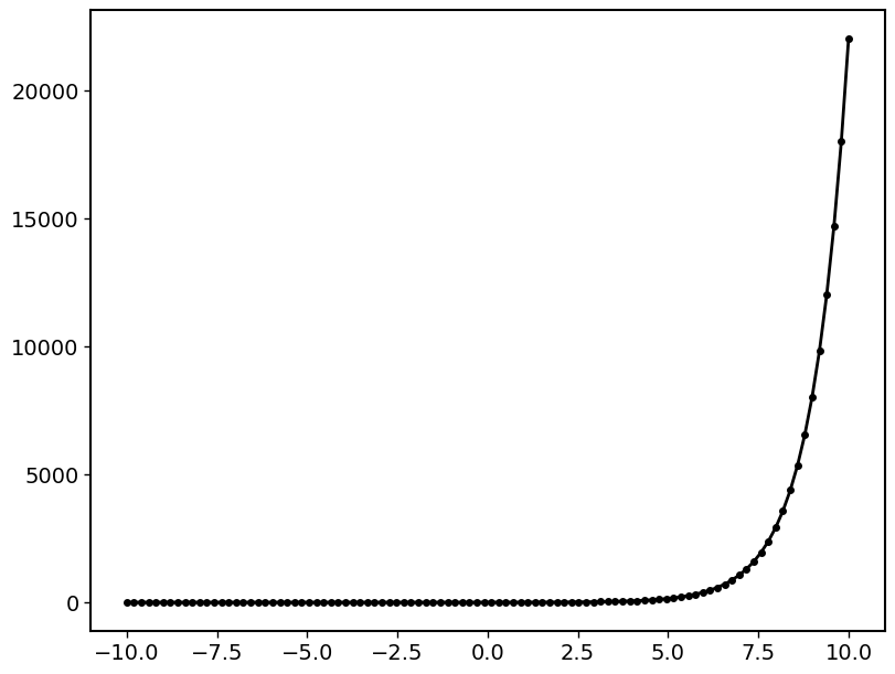
Setting limits
from masci_tools.vis.plot_methods import single_scatterplot
import numpy as np

x = np.linspace(-10, 10, 100)
y = np.exp(x)

ax = single_scatterplot(x,y, limits={'x': (-1,1), 'y': (0,4)})
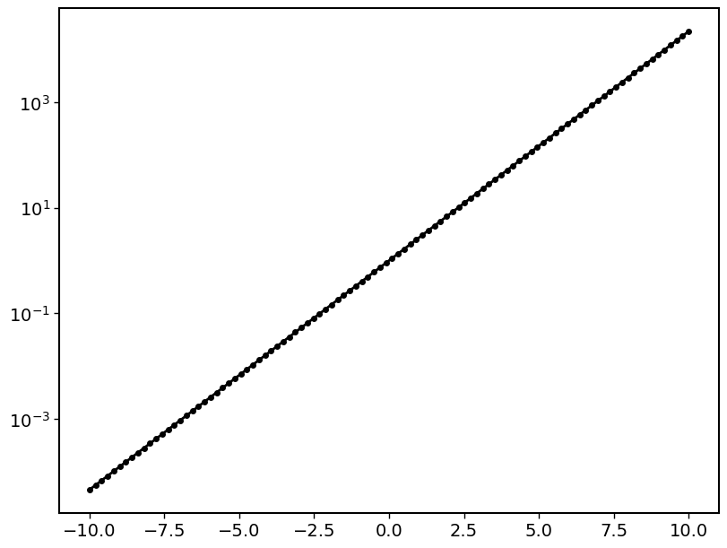
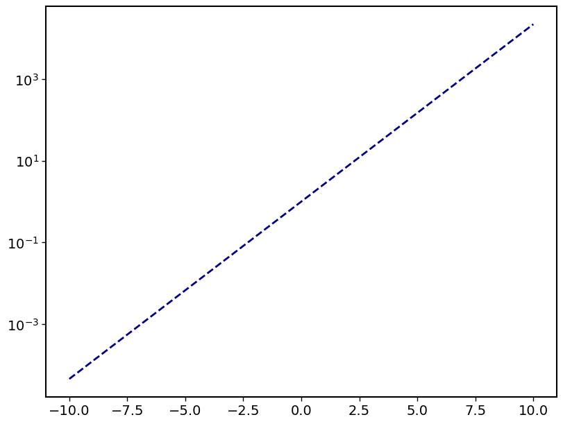
Modifying the scale of the axis
from masci_tools.vis.plot_methods import single_scatterplot
import numpy as np

x = np.linspace(-10, 10, 100)
y = np.exp(x)

ax = single_scatterplot(x,y, scale={'y': 'log'})
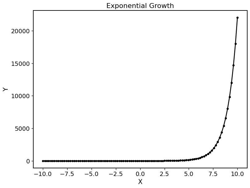
Setting labels on the axis and a title
from masci_tools.vis.plot_methods import single_scatterplot
import numpy as np

x = np.linspace(-10, 10, 100)
y = np.exp(x)

ax = single_scatterplot(x,y, xlabel='X', ylabel='Y', title='Exponential Growth')
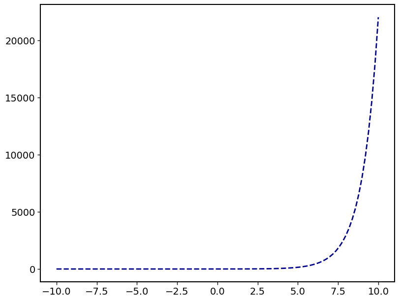
Modifying plot parameters
See the matplotlib documentation for complete references of possible options
from masci_tools.vis.plot_methods import single_scatterplot
import numpy as np

x = np.linspace(-10, 10, 100)
y = np.exp(x)

ax = single_scatterplot(x,y, color='darkblue', linestyle='--', marker=None)
Setting user defaults
If you wish to change some parameters for all the plots you want to do, you can use the
functions plot_methods.set_mpl_plot_defaults() or
bokeh_plots.set_bokeh_plot_defaults() for the matplotlib and bokeh plotting
library respectively. These functions accept the same keyword arguments as above and
they will be applied to all the next plots that you do.
You can reset the changes to the defaults with plot_methods.reset_mpl_plot_defaults()
or bokeh_plots.reset_bokeh_plot_defaults()
Note
You can still override these defaults by simply passing in another value for the parameter you wish to overwrite in the call to a plotting function
from masci_tools.vis.plot_methods import single_scatterplot, set_mpl_plot_defaults
import numpy as np

x = np.linspace(-10, 10, 100)
y = np.exp(x)

set_mpl_plot_defaults(color='darkblue', linestyle='--', marker=None)

ax = single_scatterplot(x,y, scale={'y': 'log'})
Resetting defaults:
from masci_tools.vis.plot_methods import reset_mpl_plot_defaults
reset_mpl_plot_defaults()
Multiple plots
Many plotting routines accept multiple sets of data to plot. An example of this is the
plot_methods.multiple_scatterplots() function. The usage of these is essentially
the same. However, some parameters can be changed for each data set to plot. These
include but are not limited to linestyle, linewidth, marker, markersize and color.
These parameters can either be set to a single value applying it to all data sets, or can
be specified for some/all data sets with unspecified values being replaced with the current
defaults. This second way can be done in two ways (Both of the below examples have the same
effect):
List of values (
Nonefor unspecified values) Example:linestyle=['-', None, '--']Dictionary with integer indices Example:
linestyle={0:'-', 2:'--'}
Warning
Specifying parameters for multiple data sets is only valid for the parameters passed into the function. Setting defaults with values for multiple data sets is not supported
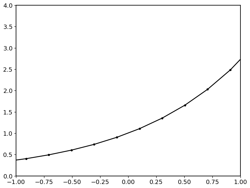
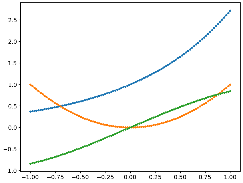
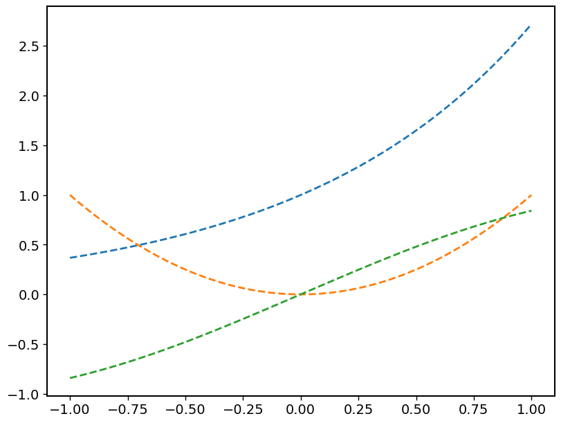
Default plot
from masci_tools.vis.plot_methods import multiple_scatterplots
import numpy as np

x = np.linspace(-1,1,100)
y = np.exp(x)
y2 = x**2
y3 = np.sin(x)

ax = multiple_scatterplots([x, x, x], [y, y2, y3])
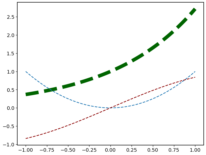
Changing parameters on all plots
from masci_tools.vis.plot_methods import multiple_scatterplots
import numpy as np

x = np.linspace(-1,1,100)
y = np.exp(x)
y2 = x**2
y3 = np.sin(x)

ax = multiple_scatterplots([x, x, x], [y, y2, y3], linestyle='--', marker=None)
Changing parameters on specific plots
from masci_tools.vis.plot_methods import multiple_scatterplots
import numpy as np

x = np.linspace(-1,1,100)
y = np.exp(x)
y2 = x**2
y3 = np.sin(x)

ax = multiple_scatterplots([x, x, x], [y, y2, y3],
                           linestyle='--',
                           marker=None,
                           color=['darkgreen', None, 'darkred'],
                           linewidth={0: 10})